on
Paper review - Design Space for Graph Neural Networks
Introduction
Design Space for Graph Neural Networks [1] was published on NeurIPS 2020. The authors are Jiaxuan You, Zhitao Ying and Jure Leskovec from Stanford. There is also a very good video from the author available on YouTube. The code is also available on Github.
Instead of evaluating a specific architecture of GNNs such as GCN, GIN or GAT, the paper explores the design space in a more general way. For example, is batch normalization helpful in GNNs? This paper answer this question empirically by performing multiple experiments.
The paper takes a systematic approach to study a general design space of GNN for many different tasks, presenting three key innovations:
- General GNN design space
- GNN task space with a similarity metric
- Design space evaluation
General GNN design space
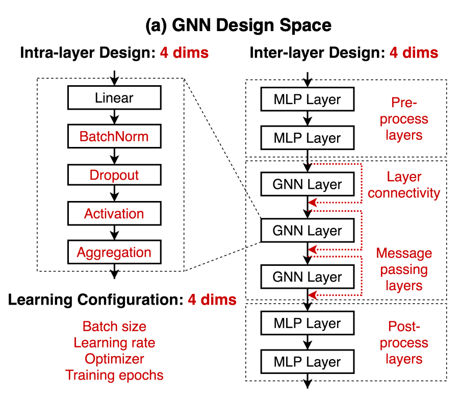
The design space is based on three configurations: intra-layer design, inter-layer design, and learning configuration. All combined possibilities result in 314,928 different designs.
 Figure 1: General design space divided into intra-layer, inter-layer and
learning configuration. Image extracted from [1].
Intra-layer design follows the sequence of the modules:
\[h^{k+1}_{v} = AGG\Big(\Big\{ACT\Big(DROPOUT(BN(W^{(k)}*h_u^{(k)} + b^{(k)}))\Big) \Big\}, u \in \mathcal{N}(v)\Big)\]It uses the following ranges:
| Aggregation | Activation | Dropout | Batch Normalization |
|---|---|---|---|
| Mean, Max, Sum | ReLU, PReLU, Swish | False, 0.3, 0.6 | True, False |
Inter-layer design is the neural network layers:
| Layer connectivity | Pre-process layers | Message passing layers | Post-precess layers |
|---|---|---|---|
| Stack, Skip-Sum, Skip-Cat | 1, 2, 3 | 2, 4, 6, 8 | 1, 2, 3 |
Training configuration is the configuration:
| Batch size | Learning rate | Optmizer | Training epochs |
|---|---|---|---|
| 16, 32, 64 | 0.1, 0.01, 0.001 | SGD, Adam | 100, 200, 400 |
I believe some of the properties selected above should not be labelled as architecture (i.e. learning rate, epochs). The talk by Ameet Talkwalkar well address the difference between hyper-parameter search and neural architecture search. Hyperparameter search starts assuming you have a fixed neural network backbone, and then there are certain properties that you want to tune. Some properties are architectural and others non-architectural:
Architectural: nodes per layer, number of layers, activation function
Non-architectural: regularization, learning rate, batch size
In NAS, you ignore the non-architectural parameters, and you also consider layer operations and networks connections in the architectural setting. Hyperparameter is the entire space to build your network, whereas neural architecture search is limited by a defined design space.
GNN task space with a similarity metric
The paper developed a technique to measure and quantify the GNN task space in conjunction with the design space. This is the most interesting idea from this paper, in my opinion, and could spawn other promising ideas. They collect 32 synthetic and real-world GNN tasks/datasets and use Kendall rank correlation [2] to compare an evaluated task to a new task. The finding is very interesting: similar tasks perform well using similar configurations, and the inverse is true. The implication is the possibility of transferring the configuration from one known task to a new task/dataset.
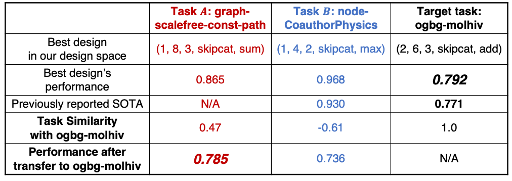
The example below demonstrates two different tasks, A and B. A controlled random search is applied to find the best design performance for each task. In this example, task A performed better using sum aggregation function, whereas task B performed better using max aggregation function. The question is if it’s possible to use the same configuration to a new similar task based on similarity.
 Table 1: Image extracted from [1]
Once introducing a new target task (ogbg-molhiv in the example), a task similarity is calculated. Task A has a correlation of 0.47, and Task B has a negative correlation of -0.61. When testing both configurations from A and B to the new task, the performance was significantly better using Task A design which has a high correlation with the target task.
Design space evaluation
The evaluation of design space alongside all the tasks lead to over 10 million possible combinations. A controlled random search is proposed to explore this space. It basically randomly sample 96 setups out of the 10M possibilities, control the configuration to be tested and evaluated. For example, consider batch normalization as the target study. A sample of 96 different configurations is randomly sampled among the design space. Batch normalization is set to True and evaluated. By preserving the other parameters, batch normalization is set to False and then evaluated again. The results are ranked by performance to generate a distribution, and the frequency is used to analyze whether batch normalization is generally helpful or not.
Experiments and Results
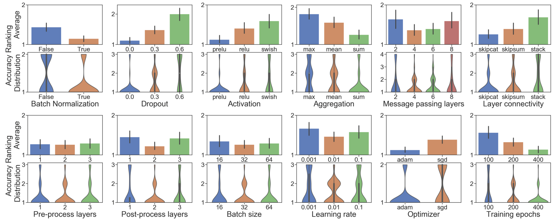
The paper show a nice visualization using violin plot for the experiments.
 Figure 3: Boxplot of the results. Image extracted from [1]
Each plot represents the distribution of the rank. For example, the first graph is the distribution of the experiments for batch normalization. By evaluating different architectures randomly, when setting batch normalization to True, it ranked better (lower is better), indicating that in most cases, the GNN will perform better when this property is used. The most expressive configurations found in this paper are:
- Dropout node feature is not effective.
- PReLU stands out as the choice of activation.
- Sum aggregation is the most expressive.
- There is no definitive conclusion for the number of message passing layers, pre-processing layers or pos-processing layers.
- Skip connections are generally favorable.
- Batch size of 32 is a safer choice, as learning rate of 0.01.
- ADAM resulted in better performance than SGD.
- More epochs of training lead to better performance.
References
- [1]J. You, R. Ying, and J. Leskovec, “Design Space for Graph Neural Networks,” 2020.
- [2]H. Abdi, The kendall rank correlation coefficient. Encyclopedia of Measurement and Statistics., 2007.